Why is reverberation time important?
The reverberation time of a room describes how long a sound “lingers” or “persists” after the source has stopped emitting it. This quality is also described a room using subjective terms such as “active”, or “live”, or “echoey”
In technical terms, the reverberation time measures rate of energy loss of a steady state sound field once the source has been shut off.
If you go into a large cathedral, one of the first things you notice is that sounds linger for a long time after they are produced. Medieval church builders deliberately aimed for this acoustic property because it perfectly suited the style of music that was to be performed there — the unaccompanied human voice singing in Latin.
Some of the best church organ music also exploits this acoustic property. For instance, think of the big pauses in the opening bars of Bach’s Toccata and Fugue in D minor. Bach was well aware of the dramatic effect the church’s acoustics could add to his music, and he exploited it!
Cathedral’s like York Minster or St Paul’s have reverberation times of in excess of 12 seconds — which is huge by modern standards. However, as music has progressed over the centuries, so the acoustics requirements of the performance spaces have changed. Modern music is usually much more rhythmical than Gregorian chant or Medieval Plain Song. This means that the buildings in which it is performed need to have much lower reverberation times, otherwise the details of the music become lost in the echoes.
Nowadays, the reverberation time of a performance space needs to fall within certain boundaries in order to be considered acceptable.
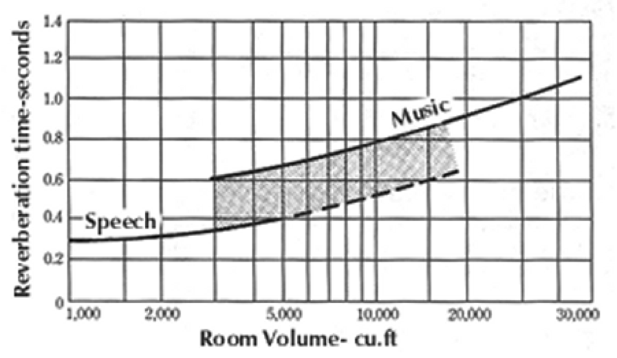
Figure 26: Acceptable reverberation times against room volume
Working with the RT60 value
The RT60 value is one of the most basic acoustic properties of a room. From this value, you can gain a first impression of the acoustic behaviour of the room as a listening environment.
Technically speaking, the RT60 value is a measure of the time taken for the energy of a particular sound impulse to drop by 60dB from its initial level. In practical terms, it is impossible to measure this drop directly due to the unavoidable presence of background noise. Therefore, a drop of 25 decibels (RT25) is measured directly and from this, the RT60 value is extrapolated. (RT60 = RT25 * 3)
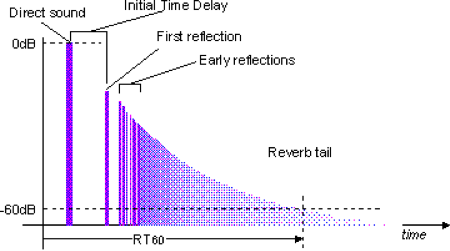
Figure 27: Echo trace showing the decay of the sound field
There is a complicating factor however! The reverberation time for a room varies depending on the frequency of the sound. Depending on the materials used in the construction of the room, it may have a long reverberation time for the bass frequencies, but a very short reverberation time for higher frequencies. This means that RT60 values must be calculated using at least 6 standard frequencies. In keeping with the tradition started by Sabine, the value at 500Hz is considered the standard RT60 value for the room.
The typical RT60 times for a small, untreated room would be presented in a table as follows:
| 64Hz | 125 Hz | 250 Hz | 500 Hz | 1 KHz | 2 KHz | 4 KHz | 8 KHz | 16 KHz |
|---|---|---|---|---|---|---|---|---|
| 1.22 | 1.06 | 0.79 | 0.61 | 0.51 | 0.48 | 0.45 | 0.39 | 0.41 |
Table 3: Reverberation times for standard measurement frequencies (shown in blue)
In this case, the room would be quoted as having an RT60 of 0.61 seconds because this is the value at 500Hz. As you can see though from the table, this room will have a problem with bass resonance.
The columns headed in blue are the standard frequencies that are always quoted for reverberation time. Those in grey are used to provide extra detail. If these values are not quoted directly, many acoustic prediction software packages will extrapolate them.
Predicting the RT60 using Sabine’s equation
A material’s absorption value is a number from 0 to 1 that indicates the proportion of sound it absorbs at a given frequency. For instance, a brick wall is a highly reflective surface, so you would expect it to absorb very little sound. In fact, the absorption value for an unpainted brick wall varies from 2% to only 7%.
The absorption values for a particular material are often quoted in a table such as the one below.
| 125 Hz | 250 Hz | 500 Hz | 1 KHz | 2 KHz | 4 KHz | |
|---|---|---|---|---|---|---|
| α | 0.02 | 0.03 | 0.03 | 0.04 | 0.05 | 0.07 |
Table 4: Absorption values for an unpainted brick wall
Mineral insulation such as fibreglass or Rockwool, on the other hand, is highly absorbent. A 25mm thick layer of fibreglass has the following absorption values:
| 125 Hz | 250 Hz | 500 Hz | 1 KHz | 2 KHz | 4 KHz | |
|---|---|---|---|---|---|---|
| α | 0.06 | 0.20 | 0.65 | 0.90 | 0.95 | 0.98 |
Table 5: Absorption values for a 25mm layer of fibreglass
As you can see from Table 5, a 25mm layer of fibreglass is a poor bass absorber, but an excellent high frequency absorber.
In order to arrive at an average absorption value for your room as a whole, Sabine developed the following procedure:
- Work out the surface area of all the different materials in the room.
- Multiply the area of each surface type by its absorbency value to give an answer in Metric Sabins. This value is also referred to as square metre absorption units (smau).
- Add up the total Metric Sabins for all the surfaces in the room. This is now the value for A in the denominator of Sabine’s equation. See Equation 18.
Worked example using Sabine’s equation
For example, a room has the following dimensions 10m x 5m x 3m (L x W x H).
Room volume = L x W x H = 10 x 5 x 3 = 150m3 Internal surface areas: Floor = L x W = 10 x 5 = 50m2 Ceiling = L x W = 10 x 5 = 50m2 Walls = 2(L x H) + 2(W x H) = 2(10 x 3) + 2(5 x 3) = 90m2 Total internal surface area = Floor + Ceiling + Walls = 50m2 + 50m2 + 90m2 = 190m2
The floor, ceiling and walls have the following respective absorbency values: 0.05, 0.7 and 0.25.
Absorption of floor = 50m2 x 0.05 = 2.5 Metric Sabins Absorption of ceiling = 50 m2 x 0.7 = 35 Metric Sabins Absorption of walls = 90 m2 x 0.25 = 22.5 Metric Sabins Total smau for the room = 2.5 + 35 + 22.5 = 60 Metric Sabins
RT60 = (0.161 * V) / A = (0.161 * 150) / 60 = 0.4s
Now putting the values for room volume and total Metric Sabins into Sabine's equation, we can obtain the following predicted reverberation time:
You have now quantified one of the basic acoustic properties of a room.
Assuming that the room for which this prediction has been made can support a well diffused sound field, then the predicted value should be close to the measured value.
You can now start to plan what form of acoustic treatment will be needed to alter the RT60 value in order to bring it into the range shown in Figure 26.
Extra information on RT60 calculations
Since Wallace Sabine derived his original equation, a lot of work has been done on closing the gap between predicted and measured RT60 values. Since Sabine’s equation is based on the assumptions that the sound field in the room is perfectly diffuse, and that the surface absorption is evenly distributed, his equation does produce reliable values for RT60 if the average absorption exceeds about 0.2.
Various modifications have been made to Sabine’s equation that all attempt to make the measured value and the predicted value match.
Norris & Eyring
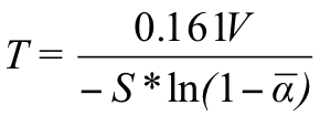
Equation 19: Norris & Eyring’s equation
Norris & Eyring used Sabine’s equation as their starting point, but took into account a property of the sound field called the “mean free path”. The mean free path is the average distance a wave front will travel in the room before it hits something.
Norris & Eyring’s equation still assumes that the room contains a completely diffuse sound field, and still requires a single, average value for the total absorbency of the room.
S is the room's total surface area and “α bar” is the room’s average absorbency.
This equation can also produce inaccurate results if one surface (typically the floor) has a significantly different absorption value from the other room surfaces.
Dariel Fitzroy
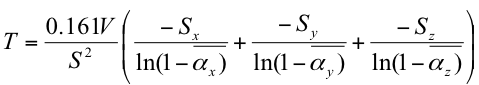
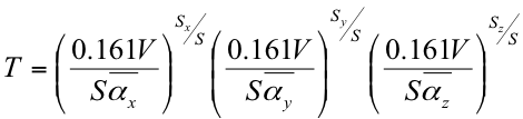
Equation 20: Fitzroy’s equation
Dariel Fitzroy was one of the first people to account for the fact that the average listening room has an uneven distribution of absorption. Typically, the floor and ceiling will be much more absorbent than the walls. This immediately reduces the level of vertical resonance, whilst making horizontal resonance more noticeable. Therefore, he improved on Norris & Eyring’s formula in order to account for this more “real-life” situation.
Fitzroy’s equation considers the absorption of each axis of the room separately. Here, Sx, Sy and Sz represent the “on-axis” surface area, and αx, αy and αz represent the “on-axis” absorption.
Higini Puchades-Arau
Equation 21: Arau’s equation
The Spanish acoustician Higini Arau has made a similar adjustment to Norris & Eyring’s formula in order to account for the fact that “real-life” rooms contain a non-uniform distribution of absorption.
Caveat
All of the formulas quoted here for calculating reverberation times take a statistical approach to solving the problem. That is, they all rely on the assumptions that:
- The energy distribution in the sound field is perfectly uniform
- The absorption is uniformly dsitributed, at least along individual axes
- That the room is rectilinear.
Failure to understand the importance of these assumptions will result in these equations being applied to situations in which one or more of the assumptions do not hold true. This will result in predictions being made that are of little or no practical value, and in a worst case, could lead a serious problem remaining undetected. For instance:
Flutter echo
A common mistake that beginners often make is to create a room in which one pair of opposing surfaces have a significantly lower absorption value than the other surfaces, E.G. absorbent walls, but a reflective floor and ceiling.
They make this mistake because the average absorption of the whole room appears to be acceptable. What has not been considered is the fact that the reflective floor and ceiling will prolong the vertical reverberation time, whilst the absorbent walls will cause the horizontal reverberation to die quickly.
This will create an effect known as a flutter echo. This is a very rapid (and annoyingly audible) sequence of echoes created by the sound resonating only in one axis.
Unfortunately, none of the quoted equations will predict this behaviour!
Avoiding flutter echo
The only way to avoid this problem is to consider the “on-axis” reverberation time. This is where you calculate the reverberation for each axis individually. Compare the following graphs:
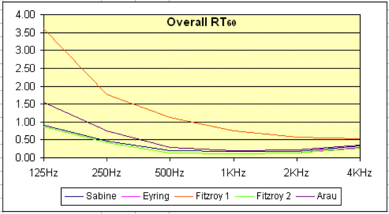
Figure 28: Graph showing overall reverberation time
This is the reverberation time graph for a small control room. The walls are made of acoustic panelling, but the floor is rough concrete, and the ceiling has been plastered. Even though Fitzroy’s equation shows a higher reverberation time, the true nature of the flutter echo is hidden from view.
Now look at a graph for the same room showing the on-axis reverberation time:
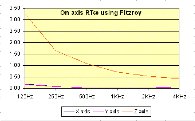
Figure 29: Graph showing on-axis reverberation time
Holy moley! Now the graph clearly shows that the Z-axis (floor-ceiling) will have a reverberation time significantly higher (at all frequencies) than the other 2 axes. If you do not consider this factor when designing your room, you may well end up making some costly (and embarrassing) mistakes!